Project name: project-gigas_ploidy
Funding source: unknown
Species: Crassostrea gigas
variable: ploidy, desiccation, high temperature
Background
After looking through the MethylKit output generated from Ronit’s samples, we are having trouble making sense of our results without the inclusion of diploid and triploid controls. To address this issue, Steven suggested that we include some of the other WGBS data we have for pacific oysters, namely from Yaamini’s Hawaii data, Roberto’s samples, and the Manchester gonad samples, as outlined within this notebook post.
Steven ran all of these through bismark and the resulting samples are stored on gannet here.
Methylkit analysis - Yaamini’s 2n/3n controls
The first thing I did was move the files Steven generated out of the scrubbed folder and into my folder
Next I ran Methylkit using this R script.
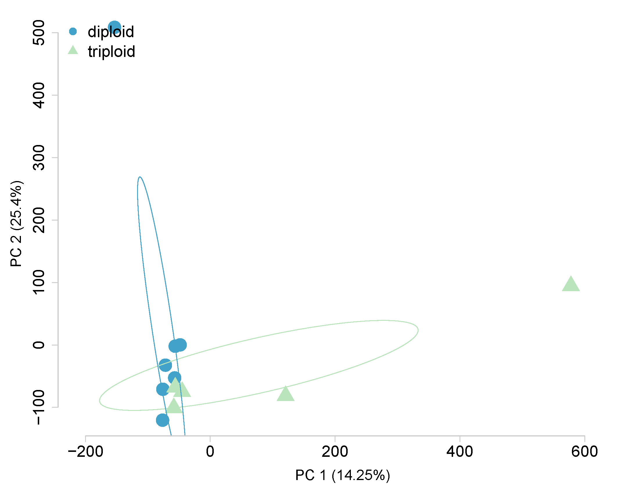
First, lets analyze just Yaamini’s controls (6 diploid and 6 triploid) to look at differences across ploidy. Using a 10x coverage, 529,068 CpGs were identified. Looking at just the impact of ploidy, the following differentially methylated loci were generated:
DMLs = 2535 identified, 1973 Hyper, 562 hypo
From here we can generate PCAs that look at the distribution of CpG and DML across ploidy.
Ploidy - All 529,068 CpGs
Ploidy - 2,535 DML only
Next, lets analyze just Ronit’s data. He has 5 diploid and 5 triploids that are both heated. Using a 10x coverage, 1,921,856 CpGs were identified. Looking at the impact of ploidy, the following differentially methylated loci were generated:
DMLs = 60,697 identified, 10,290 Hyper, 50,407 hypo
Next, lets analyze Yaamini’s samples along with Ronit’s data. Methylkit limits the comparison to CpGs that are present in both datasets, so adding them together will theoretically trim from both. Coverage files (.cov) from Bismark were processed using methRead. With both datasets together we have 22 samples (11 diploid and triploids), 10 Heated and 12 controls. Ploidy information was included in the treatment parameter using 0 = diploid, 1 = triploid.
processedFiles <- methylKit::methRead(analysisFiles,
                                      sample.id = as.list(sampleMetadata$sampleID),
                                      assembly = "Roslin",
                                      treatment = sampleMetadata$ploidyTreatment,
                                      pipeline = "bismarkCoverage",
                                      mincov = 2) #Process files. Treatment specified based on ploidy status. Use mincov = 2 to quickly process reads.
Files were then processed and filtered by 10x coverage using filterByCoverage:
processedFilteredFilesCov10 <- methylKit::filterByCoverage(processedFiles,
                                                          lo.count = 10, lo.perc = NULL,
                                                          high.count = NULL, high.perc = 99.9) %>% methylKit::normalizeCoverage(.)
The methylation information was then generated using unite:
methylationInformationFilteredCov10 <- methylKit::unite(processedFilteredFilesCov10,
                                                       destrand = FALSE,
                                                       mc.cores = 8)
This resulted in 480,579 identified methylated CpGs. Whether oysters were Heated or not was then added as a co-variate and the number of differentially methylated loci (DML, hyper and hypo) were identified using calculateDiffMeth and getMethylDiff using a 20% difference threshold:
covariateHEAT <- data.frame("HEAT" = c(rep("H", times = 10),
                                       rep("C", times = 12))) #Create dataframe with HEAT covariate information

differentialMethylationStatsPloidyCov10 <- methylKit::calculateDiffMeth(methylationInformationFilteredCov10,
                                                                   covariates = covariateHEAT).

diffMethStatsPloidyCov10Diff20 <- methylKit::getMethylDiff(differentialMethylationStatsPloidyCov10, difference = 20, qvalue = 0.01)

diffMethStats20FilteredCov10Hyper <- methylKit::getMethylDiff(differentialMethylationStatsPloidyCov10, difference = 20, qvalue = 0.01, type = "hyper")

diffMethStats20FilteredCov10Hypo <- methylKit::getMethylDiff(differentialMethylationStatsPloidyCov10, difference = 20, qvalue = 0.01, type = "hypo")
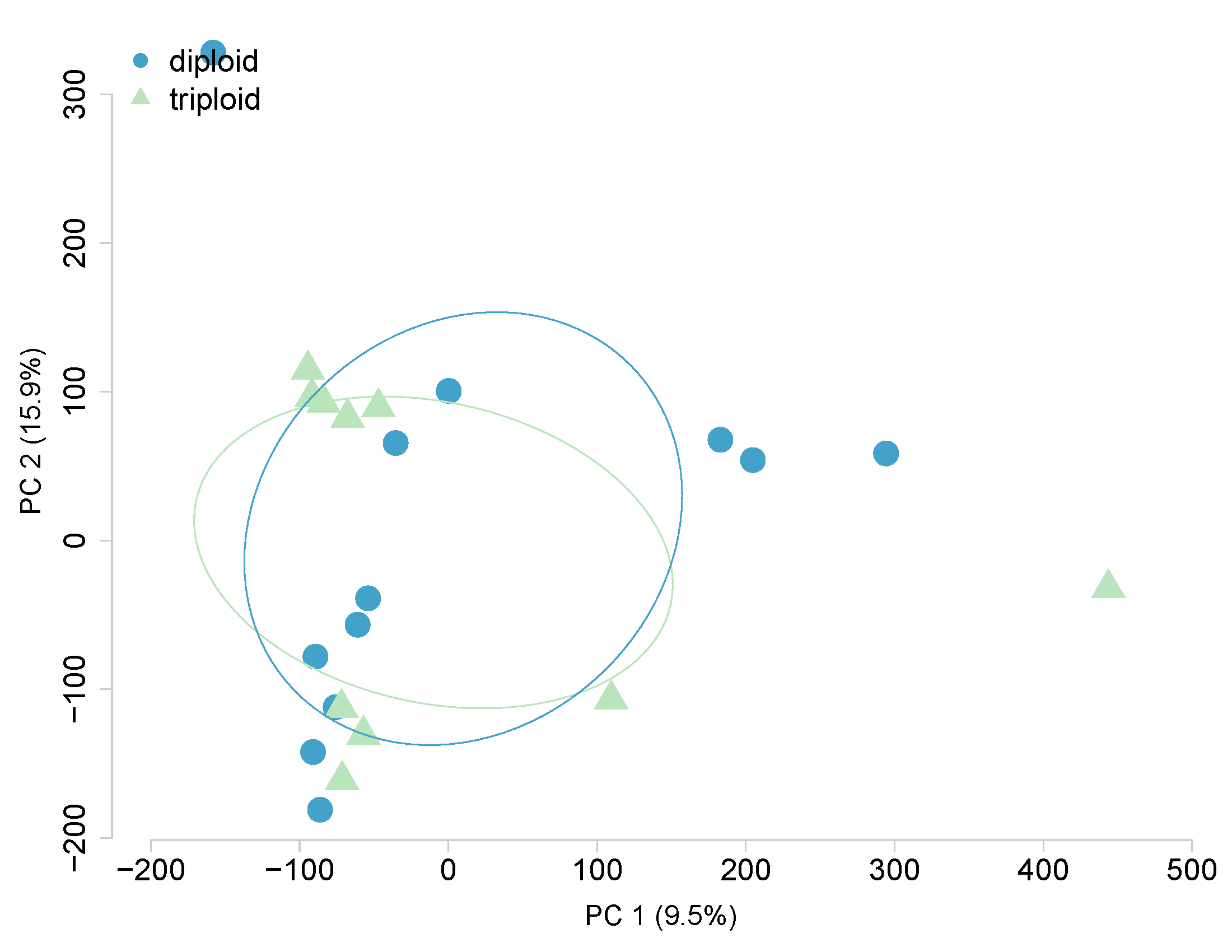
DMLs = 1038 identified, 442 Hyper, 596 hypo
From here we can generate PCAs that look at the distribution of CpG and DML across ploidy.
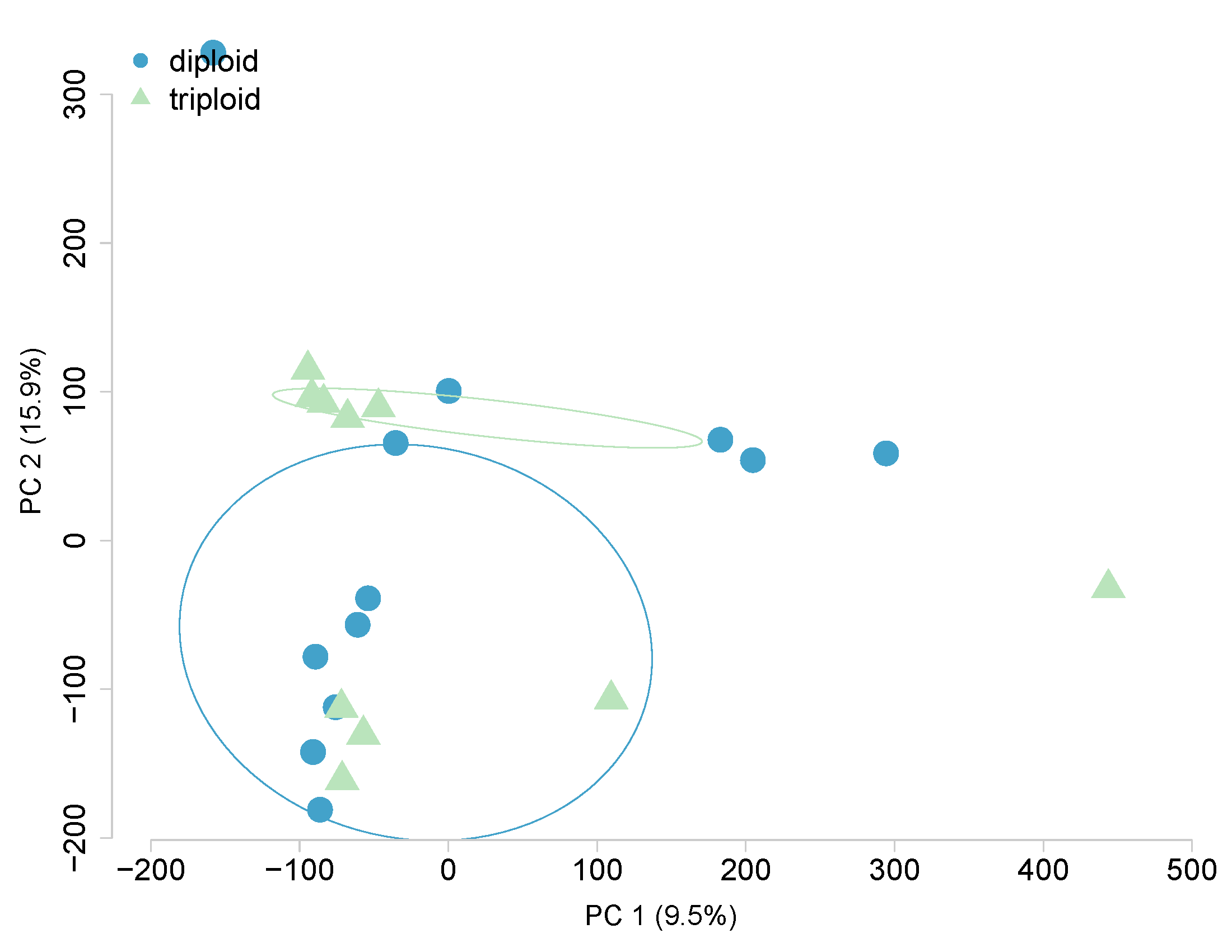
Ploidy, Heat-covariate, All 480,579 CpGs
Ploidy, Heat-covariate, 1038 DML only

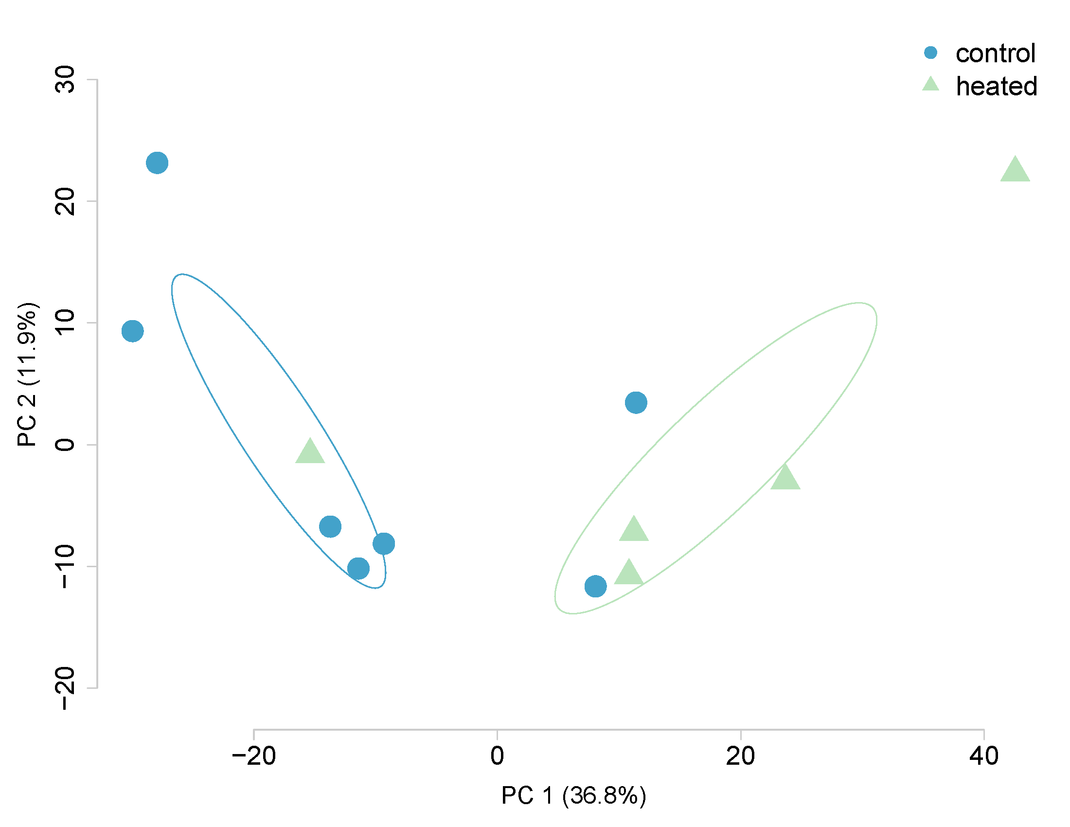
I then repeated the analysis, using HEAT as the treatment and ploidy as the covariate. The same number of CpGs were identified (480,579).
DMLs = 2351 identified, 1150 Hyper, 1201 hypo
Heated, ploidy-covariate, All 480,579 CpGs
Heated, ploidy-covariate, 2351 DML only

From all the DML tables, the following charts were then generated:
Table 1. DML counts from each analysis
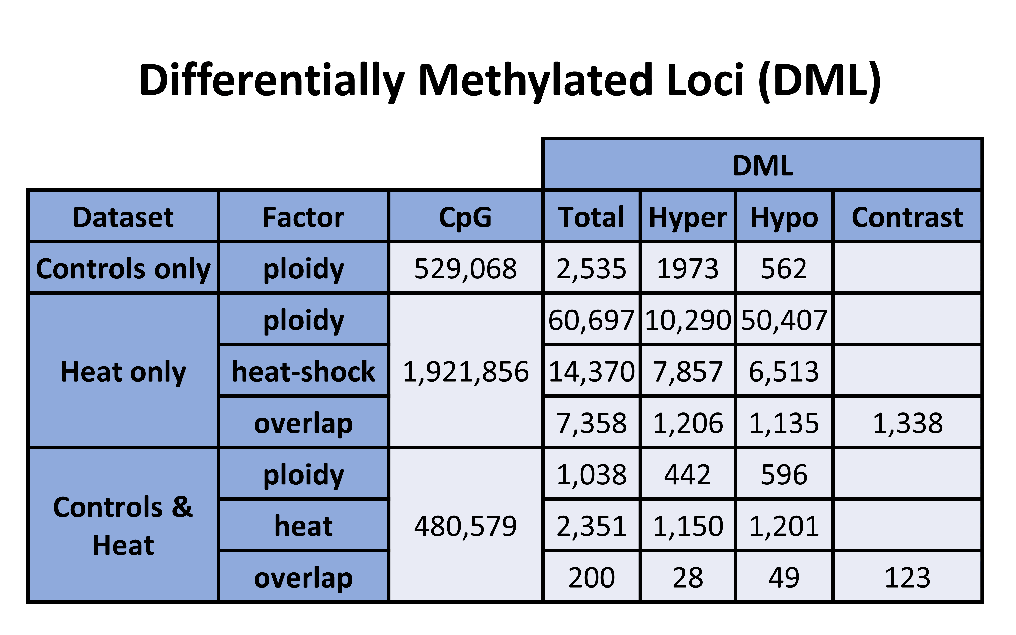
It looks like adding Ronit’s samples reduced the number of ploidy DMLs by 59.1%.
DML count comparison
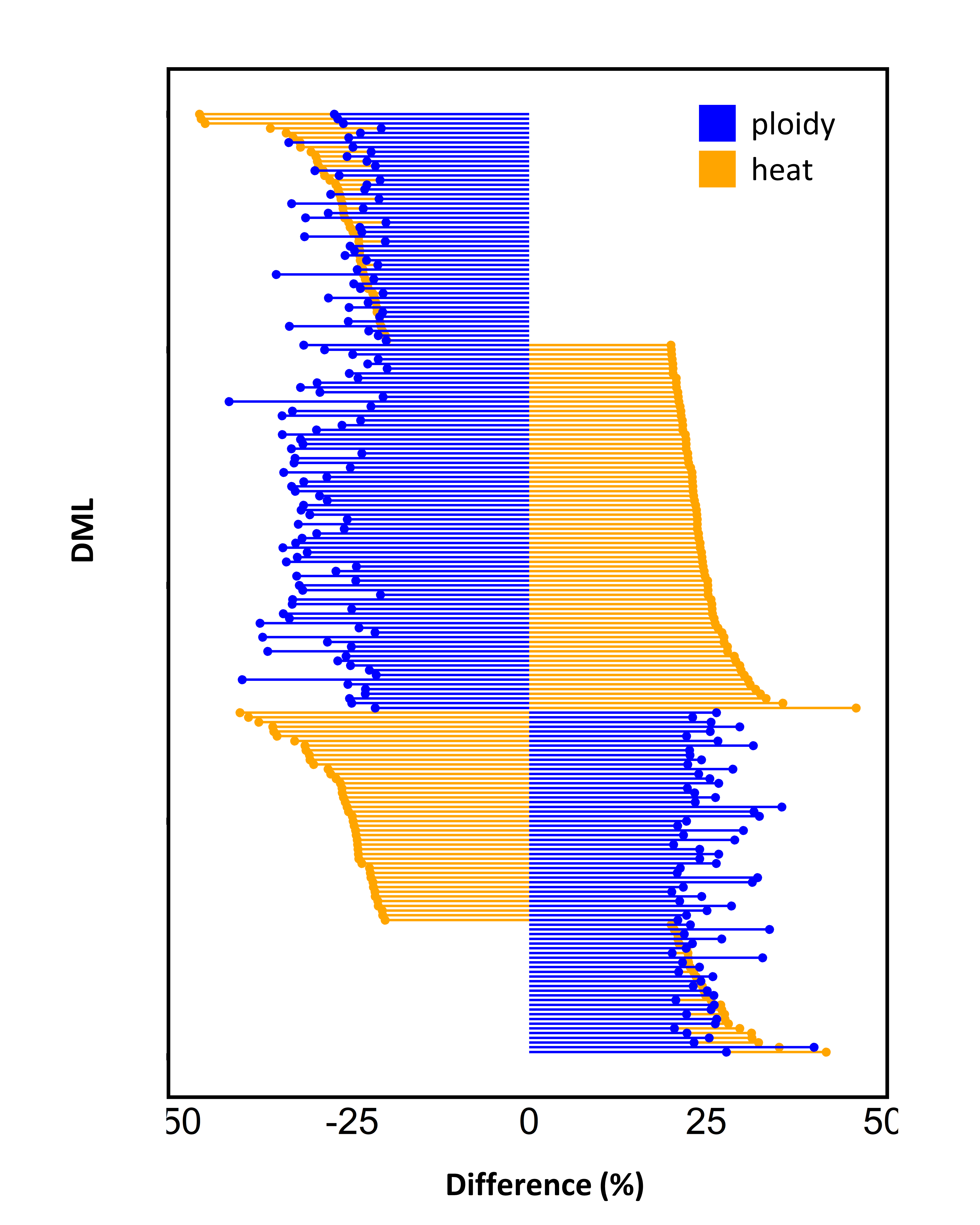
Looking at just the 200 DMLs that were in both the ploidy and heat analysis:
- 14.0% - both hypermethylated (++)
- 22.5% - ploidy hypermethylated, heat hypomethylated (+-)
- 39.0% - ploidy hypomethylated , heat hypermethylated (-+)
- 24.5% - both hypomethylated (–)