Project name: NOPP-gigas-ploidy-temp
Funding source: National Oceanographic Partnership Program
Species: Crassostrea gigas
variable: ploidy, elevated seawater temperature, desiccation
Github repo: NOPP-gigas-ploidy-temp
« previous notebook entry « | » next notebook entry »
Tagseq analysis - using HISAT2
I think I fixed the issue with low alignment scores that I was getting with HISAT2, which is a preferred aligner for TagSeq data because it is splice aware, unlike BowTie2. I hard trimmed the first 15 bp (-u 15) of the TagSeq transcripts using the following:
trim adapter sequences
mkdir trim-fastq/
cd raw-data/

for F in *.fastq
do
#strip .fastq and directory structure from each file, then
# add suffice .trim to create output name for each file
results_file="$(basename -a $F)"

# run cutadapt on each file, hard trim first 15 bp, minimum length 20
/home/shared/8TB_HDD_02/mattgeorgephd/.local/bin/cutadapt $F -a A{8} -a G{8} -a AGATCGG -u 15 -m 20 -o \
/home/shared/8TB_HDD_02/mattgeorgephd/NOPP-gigas-ploidy-temp/trim-fastq/$results_file
done
Merge, compar with MultiQC
After merging by lane, I got an average alignment rate of 72.98 +/- 3.07 sd (much better then without hard trimming ~ 55%). Here is the multiqc report for the merged, trimmed sequences.
Looking through the results, I see issues with the following samples:
D54- only 2.1 million readsN56- only 0.9 million reads, 57.6% duplicatesX44- only 1.0 million reads, 67.1% duplicates
Run DESeq2 on all, unfiltered
I ran DESeq2 on all aligned reads using this R script, without excluding samples.
Here is the pheatmap comparing all samples:

Looking at the map it looks like R53 and X42 may also be a problem, but lets run the comparisons to see if it stands out. I ran DESeq2 again, removing D54, N56, and X44 using the following R script. The analysis yielded 28,877 DEGs.
The all-treatments biplot agreed that R53 and X42 is an outlier, while also identifying M43 and N54.

Run DESeq2 w/ filters
I used the following code to filter bad/outlier samples,
coldata <- coldata[!(row.names(coldata) %in% c('D54','N56', 'X44', 'R53', 'M43', 'N54', 'X42')),]
cts <- as.matrix(subset(cts, select=-c(D54, N56, X44, R53, M43, N54, X42)))
coldata %>% dplyr::count(group)
all(colnames(cts) %in% rownames(coldata))
This resulted in at least 10 samples per treatment.
| group | ploidy | treatment | n |
|---|---|---|---|
| A | diploid | control | 11 |
| B | triploid | control | 12 |
| C | diploid | heat | 11 |
| D | triploid | heat | 10 |
| E | diploid | desiccation | 10 |
| F | triploid | desiccation | 11 |
I then ran DESeq2 on all samples, filtering by group numbers to run individual comparisons.
# Filter data
coldata_trt <- coldata # %>% filter(group == "A" | group == "B")
cts_trt     <- subset(cts, select=row.names(coldata_trt))

# Calculate DESeq object
dds <- DESeqDataSetFromMatrix(countData = cts_trt,
                              colData = coldata_trt,
                              design = ~ group)

dds <- DESeq(dds) # Run DESeq2
resultsNames(dds) # lists the coefficients
I then removed genes that didn’t have at least 1/3 of samples with 10 or more counts. See this bioconductor thread.
keep <- rowSums(DESeq2::counts(dds) >= 10) >= ncol(cts_trt)/3
dds <- dds[keep,]
Across all samples, 31,371 genes were identified and 19,089 genes were removed through filtering, resulting in 12,282 genes to compare across samples.
Here are some results:
PCA: All treatments:

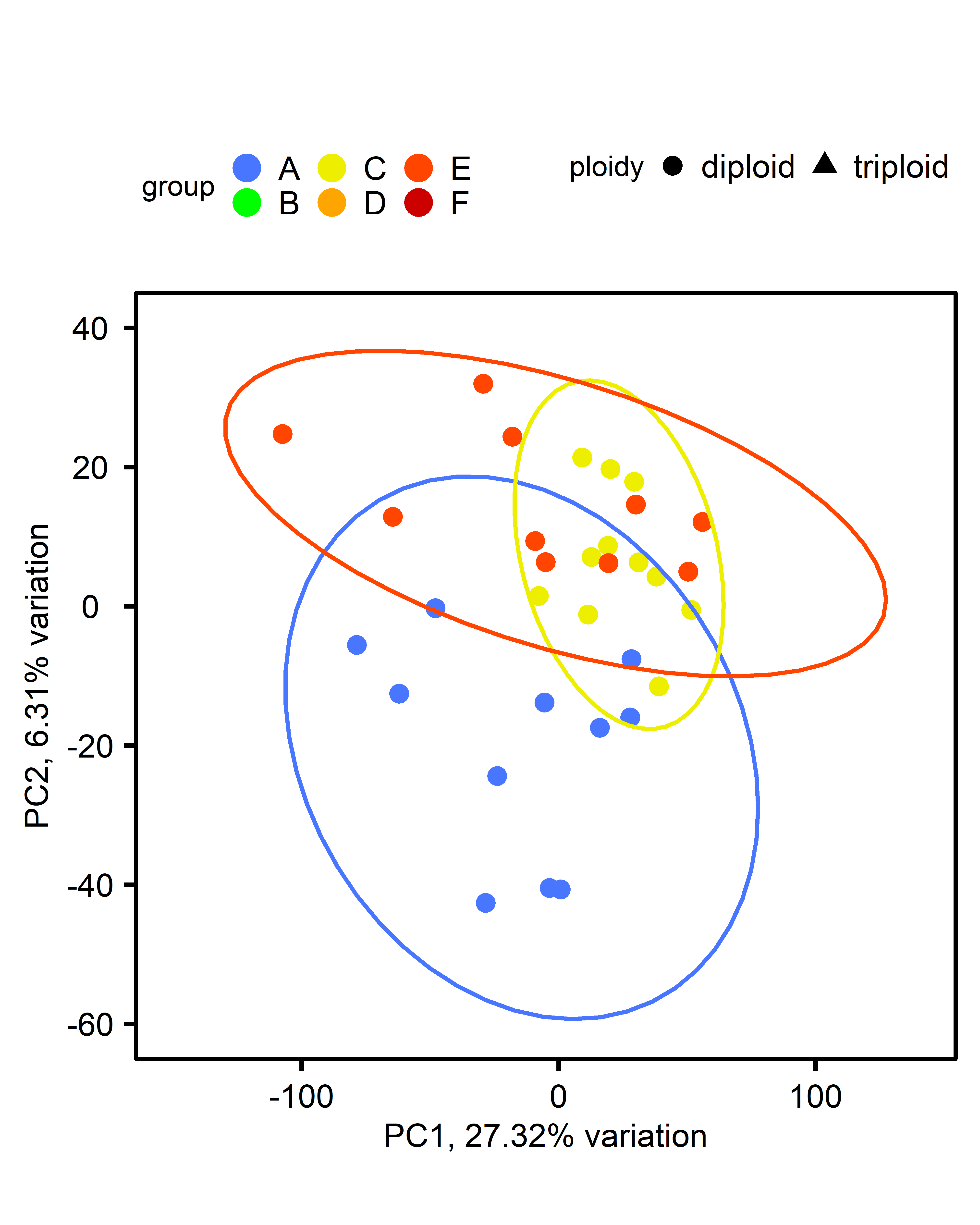
PCA: Diploid only:
PCA: Triploid only:

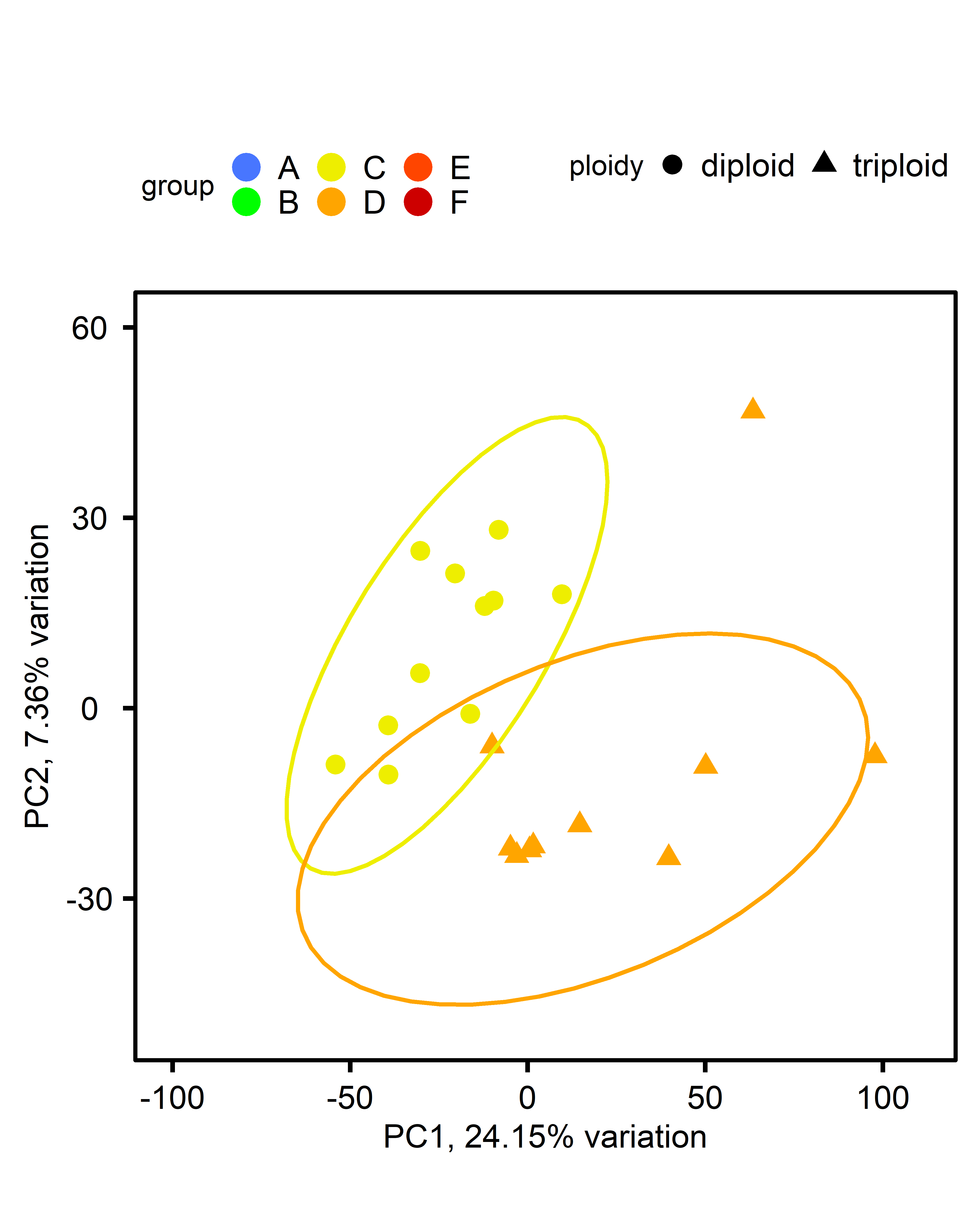
PCA: Multiple comparisons by ploidy:
| comparison | diploid | triploid |
|---|---|---|
| single-stressor v control |  |
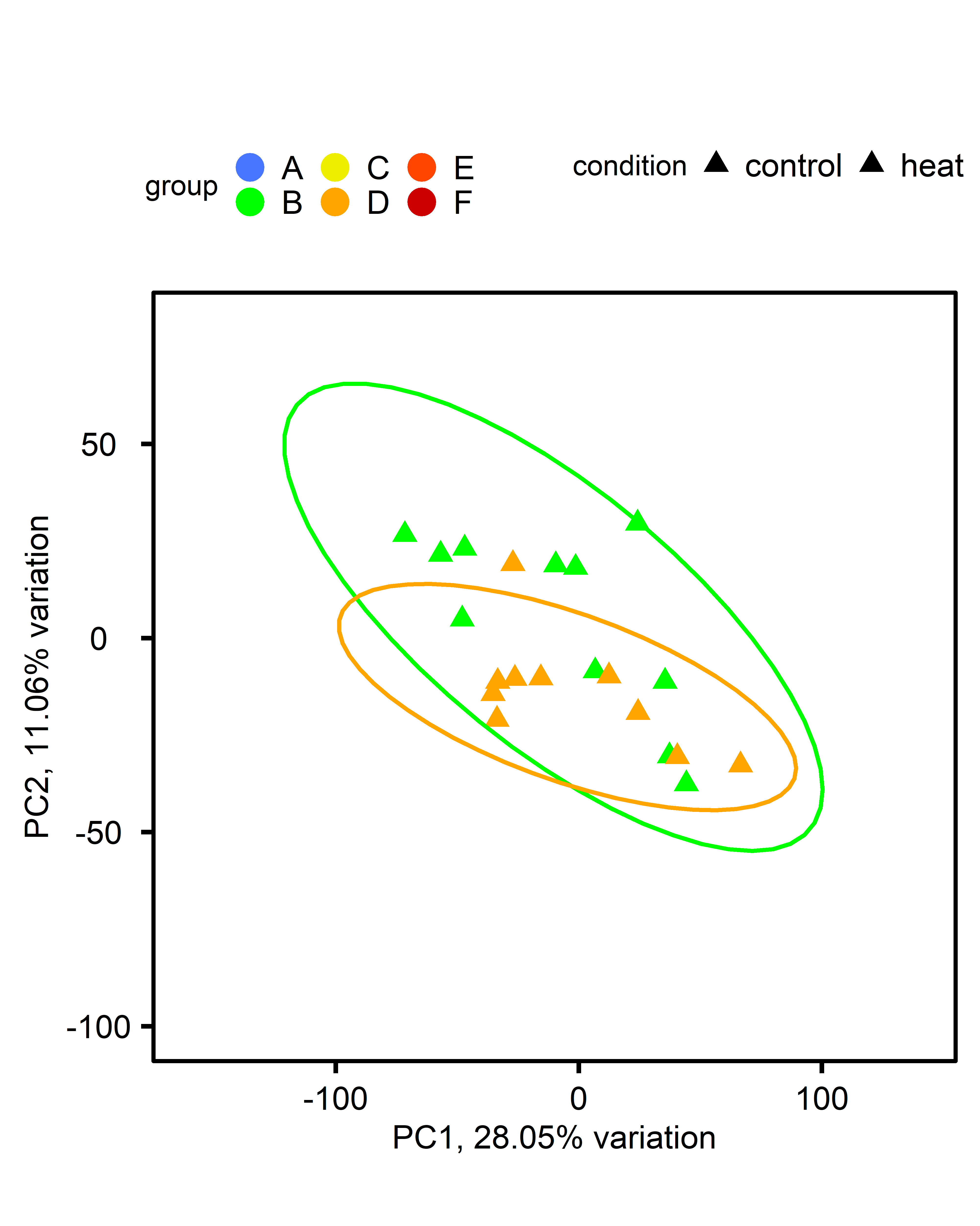 |
| multi-stressor v control | 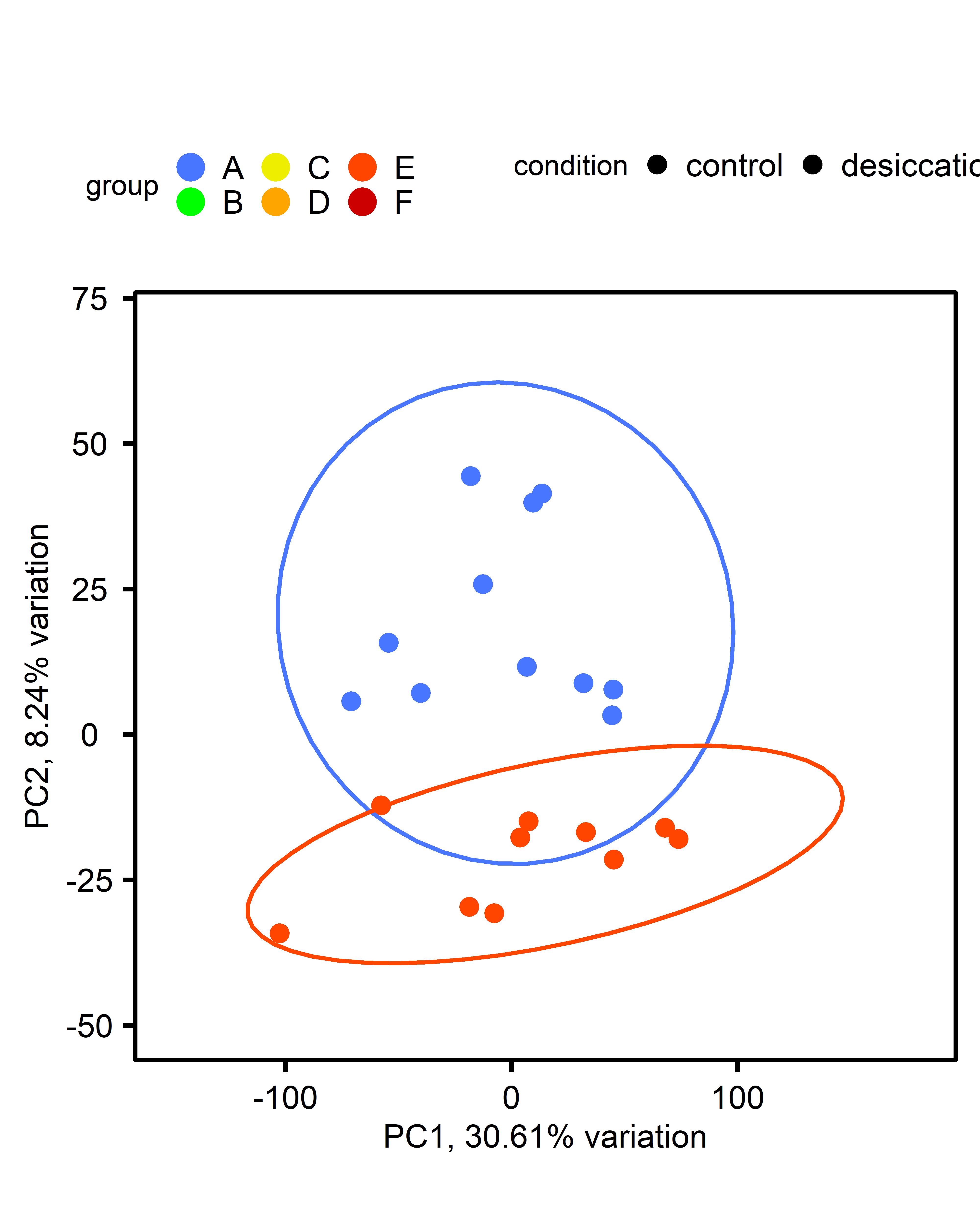 |
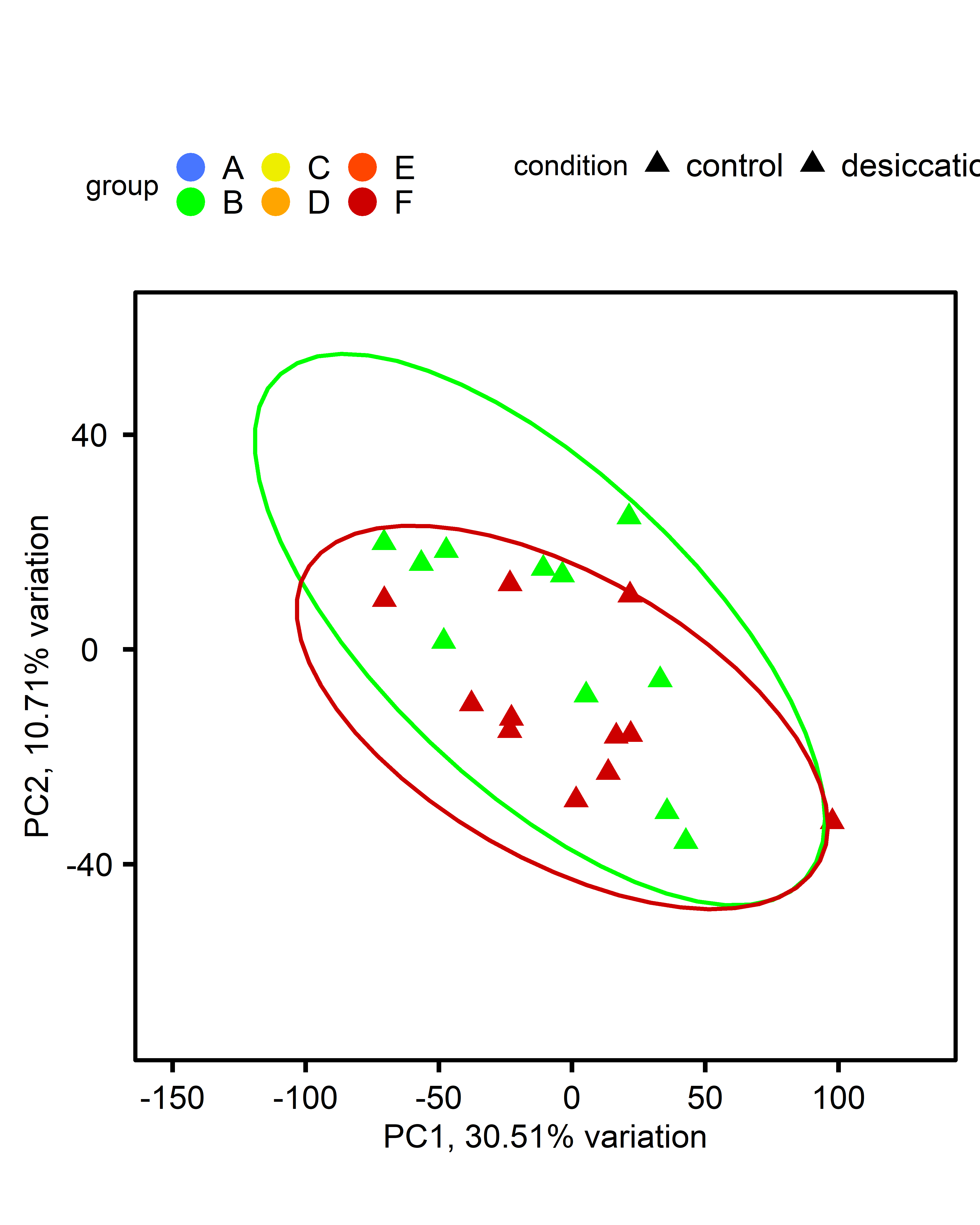 |
DEG: significant genes by treatment:
</br> Differentially expressed genes with p<0.05 and log2fold change > 1.5, using the apeglm shrinkage estimator
| comparison | diploid | triploid |
|---|---|---|
| single-stressor v control | 317 | 94 |
| multi-stressor v control | 74 | 62 |
PCA: Multiple comparisons by treatment:
| comparison | control | single-stressor | multi-stressor |
|---|---|---|---|
| ploidy |  |
 |
 |
DEG: significant genes by treatment:
Differentially expressed genes with p<0.05 and log2fold change > 1.5, using the apeglm shrinkage estimator
| comparison | control | single-stressor | multi-stressor |
|---|---|---|---|
| ploidy | 177 | 344 | 138 |